ポアソン混合モデルにおける推論 - 2. ギブスサンプリング

読書記録『機械学習スタートアップシリーズ ベイズ推論による機械学習入門』

この記事では 読書記録『機械学習スタートアップシリーズ ベイズ推論による機械学習入門』のうち、「4.3 ポアソン混合モデルにおける推論」にかんして、ギブスサンプリングによる推論を実装します。

前回の記事をお読みになってない方は、まずはそちらをご覧ください。

はじめに

この記事は、いわゆる須山ベイズ本「4.3 ポアソン混合モデルにおける推論」にかんする一連の記事のひとつです。この節での実装は

PMM.cpp
ギブスサンプリングなど推論の実装
PMM.R
推論の実行やその推論結果の可視化などの実装

の 2 つのファイルにまとめており GitHub のリポジトリ で公開しています。

各記事では、これらのファイルの該当箇所を順に説明していくかたちをとるので、関心のある方は適宜参照してください。数式やその説明をどこまで記載してよいかわからなかったので、この記事は書籍を傍らに置きながら読まれることを想定しております。

なお、改善点等ありましたらご指摘いただけると幸いです。

実装 (PMM.cpp)

準備

まずは一連の実装で必要となるライブラリを読み込みます(前回の記事に同じです)。

 1
 2
 3
 4
 5
 6
 7
 8
 9
10
11
#include <stan/math.hpp>
#include <random>
#include <string>
#include <vector>
#include <iostream>
#include <fstream>
#include <sstream>

using namespace stan;
using namespace math;
using namespace Eigen;

GibbsSampling 関数

さっそく、ギブスサンプリングを行う関数 GibbsSampling を定義します。今回は generate_data 関数(第1回の記事参照)によって生成されるデモデータに対し、ギブスサンプリングによる推論を行うため、入力として以下のものを考えます。

入力概要
N整数generate_data によって生成されたデータのサンプルサイズ
K整数クラスター数
X長さ N のベクトルgenerate_data によって生成されたデータ
MAXITER整数イテレーション数
seed整数乱数生成のためのシード値
113
114
115
116
117
118
119
120
121
122
123
124
125
126
127
128
129
130
131
132
133
134
135
136
137
138
139
140
141
142
143
144
145
146
147
148
149
150
151
152
153
154
155
156
157
158
159
160
161
162
163
164
165
166
167
168
169
170
171
172
173
174
175
176
177
178
179
180
181
182
183
184
185
186
187
188
189
190
void GibbsSampling(int N, int K, VectorXi X, int MAXITER, int seed) {
    // function to do Gibbs Sampling
    // inputs:
    //   N: the number of data points
    //   K: the number of clusters
    //   X: the data
    //   MAXITER: the maximum number of iterations
    //   seed: the random seed value
    
    // set random engine with the random seed value
    std::default_random_engine engine(seed);

    // set the output file
    std::ofstream samples("GS-samples.csv");
    // set the headers in the file
    for (int k = 0; k < K; k++) samples << "a." << k << ",";
    for (int k = 0; k < K; k++) samples << "b." << k << ",";
    for (int k = 0; k < K; k++) samples << "lambda." << k << ",";
    for (int k = 0; k < K; k++) samples << "alpha." << k << ",";
    for (int k = 0; k < K; k++) samples << "pi." << k << ",";
    for (int n = 0; n < N; n++) samples << "s." << n << ",";
    samples << "ELBO" << std::endl;

    // set variables
    VectorXd a; // the shape parameter
    VectorXd a_hat; // the modified shape parameter
    VectorXd b; // the rate parameter
    VectorXd b_hat; // the modified rate parameter
    VectorXd alpha; // the concentration parameter
    VectorXd alpha_hat; // the modified concentration parameter
    VectorXd lambda; // the rate parameter
    VectorXd pi; // the mixing parameter
    MatrixXd eta(N,K); // the temporal parameter to sample s
    VectorXi s; // the latent variable
    MatrixXi S(N,K); // the latent variable (one-hot-labeling)
    double ELBO; // ELBO

    // set initial values
    a = VectorXd::Constant(K,1,uniform_rng(0.1,2.0,engine));
    b = VectorXd::Constant(K,1,uniform_rng(0.005,0.05,engine)); 
    lambda = to_vector(gamma_rng(a,b,engine));
    alpha = VectorXd::Constant(K,1,uniform_rng(10.0,200.0,engine));
    pi = dirichlet_rng(alpha,engine);
    
    // sampling
    for (int i = 1; i <= MAXITER; i++) {
        // sample s and S
        s = VectorXi::Zero(N,1); // initialize s with zeros
        S = MatrixXi::Zero(N,K); // initialize S with zeros
        for (int n = 0; n < N; n++) {
            eta.row(n) = X(n) * log(lambda) - lambda + log(pi);
            eta.row(n) -= rep_row_vector(log_sum_exp(eta.row(n)),K);
            s(n) = categorical_rng(exp(eta.row(n)), engine);
            S(n,s(n)-1) = 1;
        }
        
        // sample lambda
        a_hat = a + S.transpose() * X;
        b_hat = b + S.colwise().sum().transpose();
        lambda = to_vector(gamma_rng(a_hat,b_hat,engine));
        
        // sample pi
        alpha_hat = alpha + S.colwise().sum().transpose();
        pi = dirichlet_rng(alpha_hat,engine);
                    
        // calc ELBO
        ELBO = calc_ELBO(N, K, X, a, b, alpha, a_hat, b_hat, alpha_hat);

        // output
        for (int k = 0; k < K; k++) samples << a_hat(k) << ",";
        for (int k = 0; k < K; k++) samples << b_hat(k) << ",";
        for (int k = 0; k < K; k++) samples << lambda(k) << ",";
        for (int k = 0; k < K; k++) samples << alpha_hat(k) << ",";
        for (int k = 0; k < K; k++) samples << pi(k) << ",";
        for (int n = 0; n < N; n++) samples << s(n) << ",";
        samples << ELBO << std::endl;
    }
}

乱数生成器と、結果を吐き出すファイル GS-samples.csv を準備したうえで変数をサンプリングしつつファイルに書き込んできます。

大まかな流れは「アルゴリズム 4.2」(書籍 p.131)にある通りで、パラメータ $\boldsymbol{\lambda}, \boldsymbol{\pi}$ に初期値を設定したうえで、各イテレーションにおいて $s_{n}, \lambda_{k}, \boldsymbol{\pi}$ を順にサンプリングしていきます。

ここでの実装では、$\boldsymbol{\lambda}, \boldsymbol{\pi}$ に初期値を設定するにあたって、 $$ \begin{align*} a &\sim \text{Uniform}(0.1,2), \\
b &\sim \text{Uniform}(0.005,0.05), \\
\alpha &\sim \text{Uniform}(10,200), \end{align*} $$ および $a_{k} = a, b_{k} = b, \alpha_{k} = \alpha\ (k = 1,\ldots, K)$ としておき、これらをもとに $\boldsymbol{\lambda}, \boldsymbol{\pi}$ を一度サンプリングしています。

残りは上述の通りで、最後に他の推論手法と比較するために ELBO を計算しています(ELBO 計算の実装は こちら)。

また、今回はギブスサンプリングということでラベルスイッチングへの対応は行っていません1

なお、筆者によるサンプルコードでは「アルゴリズム 4.2」とは違う手順をとっており、イテレーションごとの推論に入る前に $\alpha=100, a=1.0, b=0.01$ としておき、$\textbf{S}$ を初期化、それをもとに $\alpha, a, b$ を更新しています。また、イテレーションごとの推論においても、$\textbf{S}$ ではなく $\boldsymbol{\lambda}, \boldsymbol{\pi}$ からサンプリングを始めています(このことについては書籍 pp.132–133 に記載があります)。

main 関数

PMM.cpp を実行するさいに N, K, X, MAXITER, seed といった入力を渡しつつ GibbsSampling 関数を実行できるよう、main 関数を定義し、入力はコマンドライン引数として渡すことにします。

370
371
372
373
374
375
376
377
378
int main(int argc, char *argv[]) {
    
    // get inputs 1 ~ 4
    std::string method = argv[1];
    int N = atoi(argv[2]);
    int K = atoi(argv[3]);
    int seed = atoi(argv[4]);
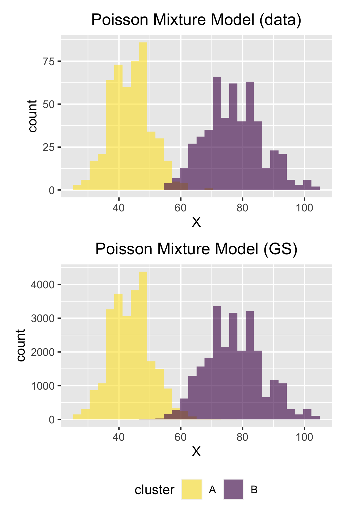
    if (method == "data") {
392
393
394
395
396
397
398
399
400
401
402
403
404
405
406
407
408
409
410
411
412
413
414
415
    } else {
        
        int MAXITER = atoi(argv[5]);

        // read data.csv
        VectorXi X;
        X = VectorXi::Zero(N);
        std::ifstream ifs("data.csv");
        std::string line;
        int idx = -1;
        while (getline(ifs, line)) {
            std::vector<std::string> strvec = split(line, ',');
            if (idx == -1) {
                idx++;
                continue;
            }
            X(idx) = stoi(strvec.at(1));
            idx++;
        }
        
        if (method == "GS") {

            std::cout << "Gibbs Sampling" << std::endl;
            GibbsSampling(N, K, X, MAXITER, seed);
431
432
433
        }
    }
}

ここで、コマンドライン引数の 1 番目として GS を受け取っており、事前に generate_data 関数で生成した data.csv を読み込んでいます。

実行 (PMM.R)

PMM.cpp をコンパイルして実行し、推論結果が確認できるように、PMM.R を実装します。

準備

(前回の記事と同じです)

 1
 2
 3
 4
 5
 6
 7
 8
 9
10
11
12
13
14
15
16
17
18
19
20
21
22
# setwd("./PoissonMixtureModel/")


# library ------------------------------
library(tidyverse)
library(colorspace)
library(patchwork)
library(ggdist)


# functions ------------------------------
make_plot <- function(method, K, s, X, bins = 30) {
  title <- str_c("Poisson Mixture Model (",method,")")
  
  tibble(s = s, X = X) %>% 
    ggplot(aes(x = X, fill = factor(s))) +
    geom_histogram(bins = bins, alpha = 0.6, position = "identity") +
    scale_fill_discrete_sequential(palette = "Viridis", labels = LETTERS[1:K]) +
    labs(title = title, fill = "cluster") +
    theme(plot.title = element_text(hjust = 0.5),
          legend.position = "bottom")
}

コンパイル

(前回の記事と同じです)

25
26
27
28
# compile c++ file ------------------------------
stan_math_standalone <- "$HOME/.cmdstanr/cmdstan-2.24.0/stan/lib/stan_math/make/standalone"
str_c("make -j4 -s -f", stan_math_standalone, "math-libs", sep = " ") %>% system()
str_c("make -j4 -s -f", stan_math_standalone, "PMM",       sep = " ") %>% system()

実行

では、次のような設定で生成されたデモデータ(第1回の記事と同じ)に対してギブスサンプリングによる推論を実行します。

入力概要
Nサンプルサイズ1000
Kクラスター数2
lambda各ポアソン分布のパラメータ44, 77
pi混合比率0.5, 0.5
seed乱数生成のためのシード値6

推論のパラメータにかんしては、デモデータと同じく N = 1000K = 2 とするとともに、seed = 1, MAXITER = 1e+2 としておき、system 関数を使って実行します。

62
63
64
65
66
67
# Gibbs Sampling ------------------------------
method <- "GS"
gs_seed <- 1
MAXITER <- 1e+2

str_c("./PMM", method, N, K, gs_seed, as.integer(MAXITER), sep = " ") %>% system()

生成されたサンプルは GS-samples.csv に保存されるので、それを読み込みます。

69
70
71
72
73
74
75
76
77
78
79
GS <- list()

# set col_types to read samples.csv
pars_type <- c("d","d","d","d","d","i","d")
pars_dim <- c(K,K,K,K,K,N,1)
col_types <- rep(pars_type, pars_dim) %>% str_c(collapse = "")

# read samples.csv
GS$samples <- 
  read_csv(file = "GS-samples.csv", col_names = TRUE, col_types = col_types) %>% 
  mutate(iteration = 1:MAXITER)

次に必要な変数 $\boldsymbol{\lambda},\boldsymbol{\pi},\textbf{S}$ を取り出します。

 62
 63
 64
 65
 66
 67
 68
 69
 70
 71
 72
 73
 74
 75
 76
 77
 78
 79
 80
 81
 82
 83
 84
 85
 86
 87
 88
 89
 90
 91
 92
 93
 94
 95
 96
 97
 98
 99
100
101
102
103
104
105
106
107
108
# calculate EAP for lambda and sort them to control the order of clusters
sorted_lambda <- 
  GS$samples %>% 
  filter(iteration >= MAXITER / 2) %>% 
  summarise(across(starts_with("lambda."), .fns = mean)) %>% 
  pivot_longer(everything()) %>% 
  pull(value) %>% 
  sort.int(index.return = TRUE)
map_s <- 1:K
names(map_s) <- sorted_lambda$ix

# pull lambda samples
GS$lambda <- 
  GS$samples %>% 
  select(iteration, starts_with("lambda.")) %>% 
  pivot_longer(cols = starts_with("lambda."),
               names_to = "k", 
               names_pattern = "lambda.([0-9]+)", 
               names_transform = list(k = as.integer),
               values_to = "lambda", 
               values_transform = list(lambda = as.double)) %>% 
  mutate(k = recode(k + 1, !!!map_s))

# pull pi samples
GS$pi <- 
  GS$samples %>% 
  select(iteration, starts_with("pi.")) %>% 
  pivot_longer(cols = starts_with("pi"),
               names_to = "k", 
               names_pattern = "pi.([0-9]+)", 
               names_transform = list(k = as.integer),
               values_to = "pi", 
               values_transform = list(pi = as.double)) %>% 
  mutate(k = recode(k + 1, !!!map_s))

# pull s samples
GS$s <- 
  GS$samples %>% 
  select(iteration, starts_with("s.")) %>% 
  pivot_longer(cols = starts_with("s."), 
               names_to = "n", 
               names_pattern = "s.([0-9]+)", 
               names_transform = list(n = as.integer),
               values_to = "s", 
               values_transform = list(s = as.integer)) %>% 
  mutate(s = recode(s, !!!map_s),
         X = demo_data$X[n+1])

なお、ラベルスイッチングへの対応として lambda に大小関係の制約を加えるといった処理を施していれば、推論結果は常に $\lambda_{1} = 44, \lambda_{2} = 77$ のように大小関係を保ったまま並びますが、今回はそういった処理を施していないため、シード値や初期値によって $\lambda_{1} = 77, \lambda_{2} = 44$ のようにも並びえます。この場合、1つ目の例でクラスター $k=1$ から発生していると推論された $x_{n}$ が、2つ目の例ではクラスター $k=2$ から発生していると推論されているだけで(たんに $k$ の値が入れ替わっただけで)、推論上なんの問題もありません。

ただ、$\lambda_{1} = 44, \lambda_{2} = 77$ としてパラメータが渡されているデモデータと比較する上では、可視化の際などに色が反転してしまって見づらくなってしまうので、「# calculate EAP for lambda and sort them to control the order of clusters」の処理では、値を昇順に並び替えるように添字を振り直しています(対応してデモデータを生成するさいには常に昇順でパラメータを与えてやる必要があります)。

さて、$\lambda_{k}$ のサンプルからその平均と、95%信頼区間を算出してみると次のようになります。

129
130
131
132
133
# Estimated lambda
GS$lambda %>% 
  filter(iteration >= MAXITER / 2) %>%
  group_by(k) %>% 
  mean_qi(lambda)
# A tibble: 2 x 7
      k lambda .lower .upper .width .point .interval
  <int>  <dbl>  <dbl>  <dbl>  <dbl> <chr>  <chr>    
1     1   43.9   43.4   44.4   0.95 mean   qi       
2     2   77.2   76.5   78.1   0.95 mean   qi  

実際の値は 44, 77 ですから、問題なく推論できていますね。

同様に $\pi_{k}$ のサンプルからその平均と、95%信頼区間を算出してみます。

135
136
137
138
139
# Estimated pi
GS$pi %>% 
  filter(iteration >= MAXITER / 2) %>%
  group_by(k) %>% 
  mean_qi(pi)
# A tibble: 2 x 7
      k    pi .lower .upper .width .point .interval
  <int> <dbl>  <dbl>  <dbl>  <dbl> <chr>  <chr>    
1     1 0.502  0.479  0.526   0.95 mean   qi       
2     2 0.498  0.474  0.521   0.95 mean   qi   

実際の値が 0.5, 0.5 ですから、こちらも問題なさそうです。

さいごに、手元のデータ $x_{n}$ に対して、推論された潜在変数 $s_{n}$ の結果を見てみます。

141
142
143
144
145
146
147
148
149
150
151
152
153
154
155
156
157
158
159
160
# plot
tmp_df <- 
  GS$s %>% 
  filter(iteration >= MAXITER / 2)
GS_plot <- 
 make_plot(
  method = method, 
  K = K,
  s = tmp_df$s,
  X = tmp_df$X,
  bins = 30
)

(
  (demo_data_plot / GS_plot) +
    plot_layout(guides = "collect") &
    theme(aspect.ratio = 0.6,
          legend.position = "bottom")
) %>% 
  ggsave(filename = "GS_result.png", width = 100, height = 150, units = "mm")
デモデータと推論結果

上の図は、ヒストグラムを描くにあたってデモデータと同じビンを設定し、各ビンに含まれている $x_{n}$ が推論を通して、各クラスターに割り当てられた回数を数えたものです。たとえば、推論が比較的難しい2つの分布の中間、x 軸上で 50 付近のデータは、デモデータ上ではすべてクラスターAに属していますが、推論の最中に何度かクラスターBに割り当てられていることがわかります。ただ、全体を通して見てみるとかなり正確に推論ができていることがわかります。

というわけで、今回はギブスサンプリングによる推論を実装しました。以降の記事では、別の手法での推論を実装し、最後に今回も計算した ELBO を使って手法間の比較をしてみます。


  1. Stan User’s Guide. 20.2 Label Switching in Mixture Models ↩︎

TELLNNN
Master’s student

My research interests include perception in human with psychophysics, EEG/MEG, or fMRI.

次へ
前へ

関連項目