ポアソン混合モデルにおける推論 - 1. デモデータの生成

読書記録『機械学習スタートアップシリーズベイズ推論による機械学習入門』

最終更新 2020/12/15 6 分で読める Book

この記事では読書記録『機械学習スタートアップシリーズベイズ推論による機械学習入門』のうち、「4.3 ポアソン混合モデルにおける推論」にかんして、デモデータの生成を実装します。

はじめに

この記事は、いわゆる須山ベイズ本「4.3 ポアソン混合モデルにおける推論」にかんする一連の記事のひとつです。この節での実装は

PMM.cpp: ギブスサンプリングなど推論の実装
PMM.R: 推論の実行やその推論結果の可視化などの実装

の 2 つのファイルにまとめており GitHub のリポジトリで公開しています。

各記事では、これらのファイルの該当箇所を順に説明していくかたちをとるので、関心のある方は適宜参照してください。数式やその説明をどこまで記載してよいかわからなかったので、この記事は書籍を傍らに置きながら読まれることを想定しております。

なお、改善点等ありましたらご指摘いただけると幸いです。

実装（PMM.cpp）

準備

まずは一連の実装で必要となるライブラリを読み込みます。

 1
 2
 3
 4
 5
 6
 7
 8
 9
10
11
#include <stan/math.hpp>
#include <random>
#include <string>
#include <vector>
#include <iostream>
#include <fstream>
#include <sstream>

using namespace stan;
using namespace math;
using namespace Eigen;

generate_data 関数

さっそく、デモデータを生成するための関数 generate_data を定義します。今回はポアソン混合モデルにしたがってデータを生成するため、入力として以下のものを考えます。

入力	型	概要
`N`	整数	サンプルサイズ
`K`	整数	クラスター数
`lambda`	長さ `K` のベクトル	各ポアソン分布のパラメータ
`pi`	長さ `K` のベクトル（総和が 1）	混合比率
`seed`	整数	乱数生成のためのシード値

13
14
15
16
17
18
19
20
21
22
23
24
25
26
27
28
29
30
31
32
33
34
35
36
37
38
39
40
void generate_data(int N, int K, VectorXd lambda, VectorXd pi, int seed) {
    // function to generate random data
    // inputs:
    //   N: the number of data points
    //   K: the number of clusters
    //   lambda: the rate parameter in poisson distribution
    //   pi: the mixing parameter
    //   seed: the random seed value

    // set random engine with the random seed value
    std::default_random_engine engine(seed);

    // set variables
    int s; // the latent variable
    int X; // the data
    
    // set the output file
    std::ofstream data("data.csv");
    // set the header in the file
    data << "s,X" << std::endl;
    for (int n = 0; n < N; n++) {
        // sample s and X
        s = categorical_rng(pi,engine);
        X = poisson_rng(lambda(s-1),engine);
        // output s and X
        data << s << "," << X << std::endl;
    }
}

for 文の中では、$x_{n}$ をサンプリングすることを考え、まずは混合比率 pi をパラメータにもつカテゴリ分布から潜在変数 s をサンプリングします。このとき、書籍では潜在変数が 1 of K (one-hot) 表現になっていますが、ここでは s は $1 \ldots K$ の値をとります。

つぎに、得られた s をもとに、$\lambda_{k}$ すなわち lambda(s-1) （zero-based のため -1）をパラメータにもつポアソン分布からデータ X をサンプリングします。

さいごに、サンプリングした s や X を data.csv に順に書き出したら完了です。

main 関数

PMM.cpp を実行するさいに N や lambda といった入力を渡しつつ generate_data 関数を実行できるよう、main 関数を定義し、入力はコマンドライン引数として渡すことにします。

370
371
372
373
374
375
376
377
378
379
380
381
382
383
384
385
386
387
388
389
390
int main(int argc, char *argv[]) {
    
    // get inputs 1 ~ 4
    std::string method = argv[1];
    int N = atoi(argv[2]);
    int K = atoi(argv[3]);
    int seed = atoi(argv[4]);

    if (method == "data") {
        
        // get parameters
        VectorXd lambda; // the rate parameter in poisson distribution
        VectorXd pi; // the mixing parameter
        lambda = VectorXd::Zero(K); // initialize with zeros
        pi = VectorXd::Zero(K); // initialize with zeros
        
        for (int k = 0; k < K; k++) lambda(k) = atof(argv[5+k]);
        for (int k = 0; k < K; k++)     pi(k) = atof(argv[5+K+k]);
        
        std::cout << "Random Data Generation" << std::endl;
        generate_data(N, K, lambda, pi, seed);

ここで、コマンドライン引数の 1 番目として method を受け取っていますが、これは実行するさいに、method として "data" を渡せばデモデータを生成し、"GS" を渡せばギブサンプリングによる推論を、"VI" を渡せば変分推論を、"CGS" を渡せば崩壊型ギブスンサンプリングによる推論を実行するように意図したものです。

それ以外のコマンドライン引数は、冒頭で説明したとおり、N、K、seed、長さ K のベクトルとして lambda および pi です。

実行 (PMM.R)

PMM.cpp をコンパイルして実行し、生成されたデモデータが確認できるように、PMM.R を実装します。

準備

ワーキングディレクトリの設定やライブラリのインポートなどは以下のとおりです。なお、サンプリング結果の可視化のため make_plot 関数を定義しています。

 1
 2
 3
 4
 5
 6
 7
 8
 9
10
11
12
13
14
15
16
17
18
19
20
21
22
# setwd("./PoissonMixtureModel/")


# library ------------------------------
library(tidyverse)
library(colorspace)
library(patchwork)
library(ggdist)


# functions ------------------------------
make_plot <- function(method, K, s, X, bins = 30) {
  title <- str_c("Poisson Mixture Model (",method,")")
  
  tibble(s = s, X = X) %>% 
    ggplot(aes(x = X, fill = factor(s))) +
    geom_histogram(bins = bins, alpha = 0.6, position = "identity") +
    scale_fill_discrete_sequential(palette = "Viridis", labels = LETTERS[1:K]) +
    labs(title = title, fill = "cluster") +
    theme(plot.title = element_text(hjust = 0.5),
          legend.position = "bottom")
}

コンパイル

PMM.cpp をコンパイルします。system 関数を使用します。

25
26
27
28
# compile c++ file ------------------------------
stan_math_standalone <- "$HOME/.cmdstanr/cmdstan-2.24.0/stan/lib/stan_math/make/standalone"
str_c("make -j4 -s -f", stan_math_standalone, "math-libs", sep = " ") %>% system()
str_c("make -j4 -s -f", stan_math_standalone, "PMM",       sep = " ") %>% system()

まずは、stan_math/make/standalone へのパスを stan_math_standalone として格納しておきます。これはお手元の環境次第だと思いますが、私は CmdStanR のものを使ったので、上のようになりました。

26 行目はどうやらセッション中に 1 度実行すればよいらしく、27 行目で PMM.cpp をコンパイルしています。

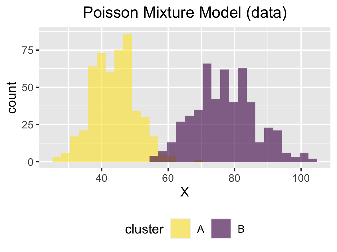
実行

ではコンパイルして得られたファイルを実行します。今回はパラメータを次のように設定しました。

入力	概要	値
`N`	サンプルサイズ	1000
`K`	クラスター数	2
`lambda`	各ポアソン分布のパラメータ	44, 77
`pi`	混合比率	0.5, 0.5
`seed`	乱数生成のためのシード値	6

コマンドライン引数が用意できたら、それらを渡しつつ system 関数を使って実行します。

31
32
33
34
35
36
37
38
39
40
41
42
43
44
# generate data ------------------------------
method <- "data"
N <- 1000
K <- 2
gen_seed <- 6

lambda <- c(44,  77)
pi     <- c(0.5, 0.5)

str_c("./PMM", method, N, K, gen_seed, 
      str_c(lambda, collapse = " "), 
      str_c(pi, collapse = " "),
      sep = " ") %>% 
  system()

今回の設定だと system 関数の入力は

./PMM data 1000 2 6 44 77 0.5 0.5

となっています。

さて、実行すると結果が格納された data.csv が生成されるので、それを読み込みます。

46
47
# read csv
demo_data <- read_csv(file = "data.csv", col_names = TRUE, col_types = "ii")

最後に読み込んだデータを可視化してみます。

49
50
51
52
53
54
55
56
57
58
59
# plot
demo_data_plot <- 
  make_plot(
    method = method,
    K = K,
    s = demo_data$s, 
    X = demo_data$X, 
    bins = 30
  )

ggsave(filename = "demo_data.png", plot = demo_data_plot, width = 100, height = 75, units = "mm")

図は載せませんが、この他にも、クラスター数を増やしたり、サンプルサイズを増やしたりすることもできます。

というわけで、今回はデモデータを生成する関数を実装しました。以降の記事ではこの関数を使って生成されたデモデータに対して推論をします。

おまけ実装 (PMM.cpp)

このままだと少し短いので、以降の記事で使用する PMM.cpp 内の関数の定義をここで紹介してしまいます。

split 関数

ひとつは、今後推論を実装するさいに、生成した data.csv を読み込むための関数です。これはほかの方の記事¹からお借りしてきたものです。

42
43
44
45
46
47
48
49
50
51
52
std::vector<std::string> split(std::string& input, char delimiter) {
    // function to get a line and split it
    // based on https://cvtech.cc/readcsv/
    std::istringstream stream(input);
    std::string field;
    std::vector<std::string> result;
    while (getline(stream, field, delimiter)) {
        result.push_back(field);
    }
    return result;
}

calc_ELBO 関数

もうひとつは、最後にギブスサンプリング、変分推論、崩壊型ギブスサンプリングを比較するさいに指標として用いられる ELBO を計算するための関数です。導出については、書籍の Appendix に記載があります。

 54
 55
 56
 57
 58
 59
 60
 61
 62
 63
 64
 65
 66
 67
 68
 69
 70
 71
 72
 73
 74
 75
 76
 77
 78
 79
 80
 81
 82
 83
 84
 85
 86
 87
 88
 89
 90
 91
 92
 93
 94
 95
 96
 97
 98
 99
100
101
102
103
104
105
106
107
108
109
110
111
double calc_ELBO(int N, int K, VectorXi X,
                 VectorXd a_pri, VectorXd b_pri, VectorXd alpha_pri,
                 VectorXd a_pos, VectorXd b_pos, VectorXd alpha_pos) {
    // function to calculate ELBO
    // inputs:
    //   N: the number of data points
    //   K: the number of clusters
    //   X: the data
    //   a_pri: the shape parameter before the update
    //   b_pri: the rate parameter before the update
    //   alpha_pri: the concentration parameter before the update
    //   a_pos: the shape parameter after the update
    //   b_pos: the rate parameter after the update
    //   alpha_pos: the concentration parameter after the update

    // calc E[lambda], E[ln lambda], and E[ln pi]
    VectorXd expt_lambda = a_pos.array() / b_pos.array();
    VectorXd expt_ln_lambda = stan::math::digamma(a_pos.array()) - stan::math::log(b_pos.array());
    VectorXd expt_ln_pi = stan::math::digamma(alpha_pos.array()) - stan::math::digamma(stan::math::sum(alpha_pos.array()));

    // calc E[ln eta], E[S], E[ln S]
    // S is a variable translated from s with one-hot-labeling
    MatrixXd expt_ln_eta(N,K);
    MatrixXd expt_ln_S(N,K);
    MatrixXd expt_S(N,K);
    for (int n = 0; n < N; n++) {
        expt_ln_eta.row(n) = X(n) * expt_ln_lambda - expt_lambda + expt_ln_pi;
        expt_ln_eta.row(n) = expt_ln_eta.row(n) - rep_matrix(stan::math::log_sum_exp(expt_ln_eta.row(n)),1,K);
        expt_ln_S.row(n) = expt_ln_eta.row(n);
    }
    expt_S = exp(expt_ln_S);

    // calc log-likelihood
    double expt_ln_lkh = 0;
    for (int n = 0; n < N; n++) {
        expt_ln_lkh += expt_S.row(n) * (X(n) * expt_ln_lambda - expt_lambda - rep_matrix(stan::math::lgamma(X(n)+1),K,1));
    }
    
    // calc E[ln p(S)] and E[ln q(S)]
    double expt_ln_pS = sum(expt_S * expt_ln_pi);
    double expt_ln_qS = sum(expt_S.array() * expt_ln_S.array());

    // calc KL[q(lambda) || p(lambda)]
    double KL_lambda = stan::math::sum(
        a_pos.array() * log(b_pos.array()) - a_pri.array() * log(b_pri.array()) -
        stan::math::lgamma(a_pos.array()) + stan::math::lgamma(a_pri.array()) +
        (a_pos.array() - a_pri.array()) * expt_ln_lambda.array() +
        (b_pri.array() - b_pos.array()) * expt_lambda.array()
    );

    // calc KL[q(pi) || p(pi)]
    double KL_pi = 
        stan::math::lgamma(sum(alpha_pos)) - stan::math::lgamma(sum(alpha_pri)) -
        sum(stan::math::lgamma(alpha_pos)) + sum(stan::math::lgamma(alpha_pri)) +
        (alpha_pos - alpha_pri).transpose() * expt_ln_pi;
    
    return expt_ln_lkh + expt_ln_pS - expt_ln_qS - (KL_lambda + KL_pi);
}

C++でCSVファイルを読み込む ↩︎

Bayes Machine Learning C++ R

ポアソン混合モデルにおける推論 - 1. デモデータの生成

はじめに

実装（PMM.cpp）

準備

generate_data 関数

main 関数

実行 (PMM.R)

準備

コンパイル

実行

おまけ実装 (PMM.cpp)

split 関数

calc_ELBO 関数

TELLNNN

Master’s student

関連項目

ポアソン混合モデルにおける推論 - 1. デモデータの生成

はじめに

実装 （PMM.cpp）

準備

generate_data 関数

main 関数

実行 (PMM.R)

準備

コンパイル

実行

おまけ実装 (PMM.cpp)

split 関数

calc_ELBO 関数

TELLNNN

Master’s student

関連項目

実装（PMM.cpp）