この記事では
読書記録『機械学習スタートアップシリーズ ベイズ推論による機械学習入門』のうち、「4.3 ポアソン混合モデルにおける推論」にかんして、ギブスサンプリングによる推論、変分推論、崩壊型ギブスサンプリングによる推論の比較を実装します。
前回の記事をお読みになってない方は、まずはそちらをご覧ください。
はじめに
この記事は、いわゆる須山ベイズ本「4.3 ポアソン混合モデルにおける推論」にかんする一連の記事のひとつです。この節での実装は
- PMM.cpp
- ギブスサンプリングなど推論の実装
- PMM.R
- 推論の実行やその推論結果の可視化などの実装
の 2 つのファイルにまとめており
GitHub のリポジトリ で公開しています。
各記事では、これらのファイルの該当箇所を順に説明していくかたちをとるので、関心のある方は適宜参照してください。数式やその説明をどこまで記載してよいかわからなかったので、この記事は書籍を傍らに置きながら読まれることを想定しております。
なお、改善点等ありましたらご指摘いただけると幸いです。
実行 (PMM.R)
今回は、新たにデモデータを 1 セット作成し、それに対するギブスサンプリングによる推論、変分推論、崩壊型ギブスサンプリングによる推論を繰り返し行い、ELBO を指標に手法間の比較を行います。
準備
(前回の記事と同じです)
 1
 2
 3
 4
 5
 6
 7
 8
 9
10
11
12
13
14
15
16
17
18
19
20
21
22
| # setwd("./PoissonMixtureModel/")
# library ------------------------------
library(tidyverse)
library(colorspace)
library(patchwork)
library(ggdist)
# functions ------------------------------
make_plot <- function(method, K, s, X, bins = 30) {
title <- str_c("Poisson Mixture Model (",method,")")
tibble(s = s, X = X) %>%
ggplot(aes(x = X, fill = factor(s))) +
geom_histogram(bins = bins, alpha = 0.6, position = "identity") +
scale_fill_discrete_sequential(palette = "Viridis", labels = LETTERS[1:K]) +
labs(title = title, fill = "cluster") +
theme(plot.title = element_text(hjust = 0.5),
legend.position = "bottom")
}
|
コンパイル
(前回の記事と同じです)
25
26
27
28
| # compile c++ file ------------------------------
stan_math_standalone <- "$HOME/.cmdstanr/cmdstan-2.24.0/stan/lib/stan_math/make/standalone"
str_c("make -j4 -s -f", stan_math_standalone, "math-libs", sep = " ") %>% system()
str_c("make -j4 -s -f", stan_math_standalone, "PMM", sep = " ") %>% system()
|
実行
では、次のような設定でデモデータを生成します。
| 入力 | 概要 | 値 |
|---|
N | サンプルサイズ | 1000 |
K | クラスター数 | 8 |
lambda | 各ポアソン分布のパラメータ | 10, 50, 90, 130, 170, 210, 250, 290 |
pi | 混合比率 | 0.125, 0.125, 0.125, 0.125, 0.125, 0.125, 0.125, 0.125 |
seed | 乱数生成のためのシード値 | 3 |
329
330
331
332
333
334
335
336
337
338
339
340
341
342
| # 手法間の比較 ------------------------------
method <- "data"
N <- 1000
K <- 8
gen_seed <- 3
lambda <- seq(10, 40 * K, by = 40)
pi <- rep(1/K, K)
str_c("./PMM", method, N, K, gen_seed,
str_c(lambda, collapse = " "),
str_c(pi, collapse = " "),
sep = " ") %>%
system()
|
生成したデモデータを読み込み、可視化してみます。
344
345
346
347
348
349
350
351
352
353
354
355
356
357
| # read csv
demo_data <- read_csv(file = "data.csv", col_names = TRUE, col_types = "ii")
# plot
data_plot_comparison <-
make_plot(
method = method,
K = K,
s = demo_data$s,
X = demo_data$X,
bins = 30
)
ggsave(filename = "comparison_data.png", plot = data_plot_comparison, width = 160, height = 100, units = "mm")
|
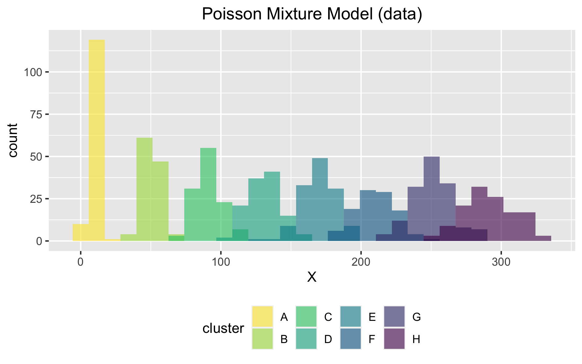 デモデータ
デモデータ推論に入る前に、データの読み込みのための準備をしておきます。
359
360
361
362
363
364
365
366
367
368
369
370
371
372
373
| # set col_types
col_types_list <- list(GS = NULL, VI = NULL, CGS = NULL)
pars_type <- c("-","-","-","-","-","-","d")
pars_dim <- c(K,K,K,K,K,N,1)
col_types <- rep(pars_type, pars_dim) %>% str_c(collapse = "")
col_types_list$GS <- col_types
col_types_list$VI <- col_types
pars_type <- c("-","-","-","-","d")
pars_dim <- c(K,K,K,N,1)
col_types <- rep(pars_type, pars_dim) %>% str_c(collapse = "")
col_types_list$CGS <- col_types
|
それでは上のようなデモデータに対し、各手法による推論を 5 回ずつ繰り返します。
推論のパラメータにかんしては、手法によらず、N = 1000、K = 8(デモデータに同じ)とするとともに、seed = 1, 2, 3, 4, 5(反復の回数)、MAXITER = 1e+4 とします。
各推論の初期値はランダムに決まるようにしてあるので、seed の値によって異なる初期値から推論が開始されます。
375
376
377
378
379
380
381
382
383
384
385
386
387
388
389
390
391
392
393
394
395
396
397
398
399
| # repetitions
N_rep <- 5
N <- 1000
K <- 8
MAXITER <- 1e+4
sim_res <- list(GS = list(), VI = list(), CGS = list())
for (method in names(sim_res)) {
for (i in 1:N_rep) {
sprintf("i = %i ", i) %>% cat()
str_c("./PMM", method, N, K, i, as.integer(MAXITER), sep = " ") %>% system()
# read samples.csv
sim_res[[method]][[i]] <-
str_c(method, "-samples.csv") %>%
read_csv(file = .,
col_names = TRUE,
col_types = col_types_list[[method]],
progress = FALSE) %>%
mutate(iteration = 1:n())
}
sim_res[[method]] <-
bind_rows(sim_res[[method]], .id = "rep")
}
|
さて、手法間の比較の指標として ELBO を採用していますが、5 回の反復における平均も計算しておきます。
401
402
403
404
405
406
407
408
409
410
| averaged_sim_res <-
sim_res %>%
map(.f = ~{
.x %>%
group_by(iteration) %>%
summarise(ELBO = mean(ELBO), .groups = "drop") %>%
mutate(rep = "averaged")
}
) %>%
bind_rows(.id = "method")
|
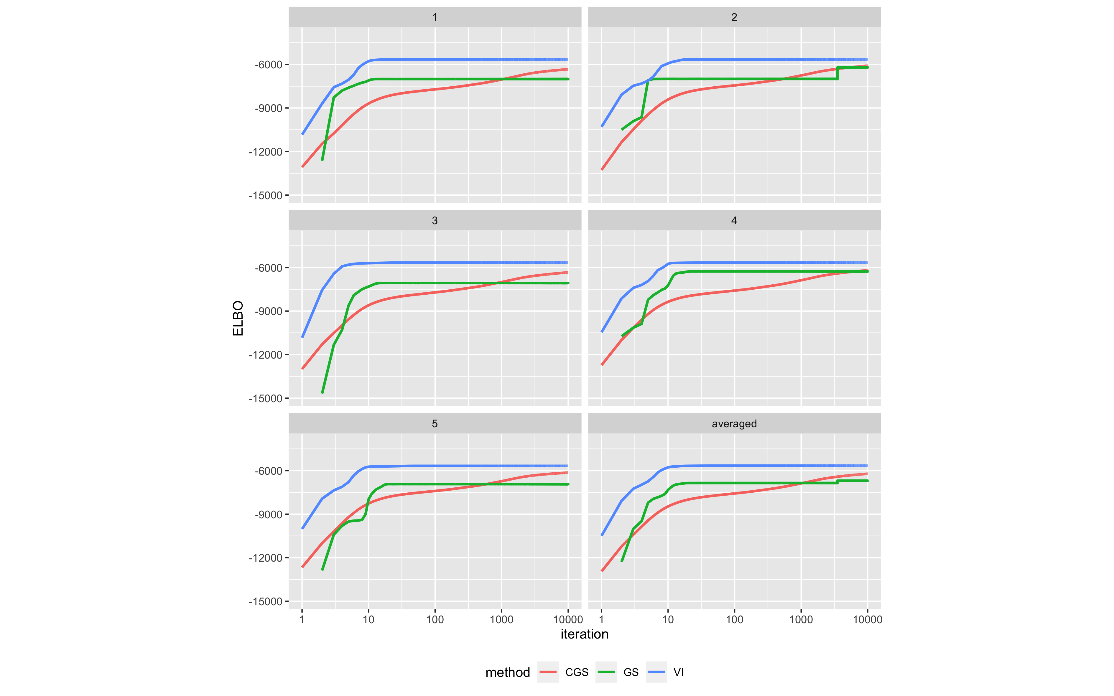
それでは、ついに、イテレーションの増加に伴う ELBO の値の変化を手法間で比較してみます。
412
413
414
415
416
417
418
419
420
421
422
423
424
| plot_comparison <-
sim_res %>%
bind_rows(.id = "method") %>%
bind_rows(averaged_sim_res) %>%
ggplot(aes(x = iteration, y = ELBO, color = method)) +
facet_wrap(. ~ rep, nrow = 3, ncol = 2) +
geom_line(size = 1) +
scale_x_continuous(trans = "log10") +
scale_y_continuous(limits = c(-15e+3,-4e+3)) +
theme(aspect.ratio = 0.6,
legend.position = "bottom")
ggsave(filename = "comparison_result.png", plot = plot_comparison, width = 320, height = 200, units = "mm")
|
 手法間の比較結果(クリックして拡大)
書籍にもあるとおり、変分推論は初期段階での高速な収束性能を示しています。また、ギブスサンプリングおよび崩壊型ギブスサンプリングによる推論の方が変分推論よりも最終的な推論結果がよくなる傾向にあるとの記述がありますが、確かにイテレーションが増えるにつれて変分推論の水準へと近づく様子が見て取れます。上の図では変分推論が最も良く見えますが、たとえばイテレーション数をさらに増やした場合には(崩壊型)ギブスサンプリングによる手法の方が追い越すことが期待されます。
さて、この記事をもって、
読書記録『機械学習スタートアップシリーズ ベイズ推論による機械学習入門』のうち、「4.3 ポアソン混合モデルにおける推論」にかんする実装は以上になります。